Message Passing on Clustered Graphs
Message passing on clustered networks with edge-disjoint clique covers using `gcmpy`
1
2
3
4
5
6
7
8
9
10
 import ast
import gcmpy
import numpy as np
import networkx as nx
import itertools
from tqdm import tqdm
from joblib import Parallel, delayed

import matplotlib
from matplotlib import pyplot as plt
[Peter Mann, 2022, University of St Andrews]
Message passing on clustered networks
In this notebook we will study bond percolation over a coauthorship network, an empirical network of condensed matter physics coauthors [1]. We will do this by solving message passing equations. This network is known to contain short loops, and so, can be challenging to solve analytically due to correlations among the message passing equations. To write our message passing expressions, we will use recent theoretical results [2] in conjunction with an edge-disjoint clique cover. We will use some of the features of gcmpy, a Python library for working with the configuration model and other network science related tools.
# Read in the network from a GML file
H = nx.read_gml("cond-mat/cond-mat.gml")

# pull the largest connected component as a networkx object
Gcc: list = list(sorted(nx.connected_components(H), key=len, reverse=True))
G = H.subgraph(Gcc[0])

# relabel the vertices with integers
G = nx.convert_node_labels_to_integers(G)
Monte Carlo simulation
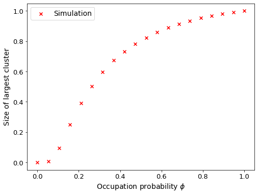
To start out, lets perform some bond percolation simulations over this network using gcmpy’s bond_percolate() routine and visualise the results.
# set the number of repeats and perform the experiments
repeats = 10
Ss = [[gcmpy.bond_percolate(G, phi) for phi in np.linspace(0,1,20)]
                                    for r in tqdm(range(repeats))]

# take the average of the repeats
largest_component_size = [sum(t)/len(t) for t in zip(*Ss)]

# plot the results
ax = plt.figure(figsize=(8,6),linewidth=7).gca()
ax.scatter(np.linspace(0,1,len(largest_component_size)),
           largest_component_size,marker='x',color='r',zorder=100,label='Simulation')

plt.xlabel(r'Occupation probability $\phi$',fontsize=14)
ax.set_ylabel('Size of largest cluster',fontsize=14)
ax.tick_params(axis='both', which='major', labelsize=13)
plt.legend(fontsize=14)

Message passing model
Now, we would like to create an analytical model using message passing. The first step is to cover the network in cliques, such that each edge belongs to a single clique. There are multiple ways to do this and gcmpy provides a few different methods (see EECC() and MPCC()) [3,4]. Today, we will use the MPCC which stands for motif preserving clique cover [3]. This method finds all of the cliques in a network, placing them into a list; orders them by size before shuffling the list of cliques that have equal size. The list is then iterated such that the largest cliques are first, and for each clique $c$ attempts to include it into the cover $\mathcal C$. A clique can be included in $\mathcal C$ iff all of its edges are available - this is the edge disjoint property. If the clique is included, its edges are marked as unavailable and the next clique is tested. This way, overlapping cliques (that share an edge) cannot both be placed in the cover.
The size of the largest connected component $S$ following bond percolation in the message passing model is given by [2]
\[S(\phi) = 1 - \frac{1}{N}\sum_i\prod _{\tau\in\tau_i} H_{i\leftarrow \tau}(1)\]The expression to calculate the clique equation is found to be [2]
\[H_{i\leftarrow \tau}(z) = \sum_{\kappa=0}^{|\tau|-1}\sum_{m=0}^{\frac 12 \kappa(\kappa-1)}\mathcal Q_{\kappa+1,\frac 12(\kappa+1)\kappa-m}\phi^{\frac 12(\kappa+1)\kappa-m}(1-\phi)^{\omega(r)+m}\sum_{a_{\kappa}\in A_{\kappa}}\prod_{\tau_j\in a_\kappa}\left(z\prod_{\nu\in \nu_{\tau_j}\backslash\tau} H_{\tau_j\leftarrow\nu}(z)\right),\]where $\mathcal Q_{n,k}$ is the number of connected graphs with $n$ vertices and $k$ edges. This can be evaluated numerically by a fast recursive algorithm due to Harary and Palmer [5].
\[\mathcal Q_{n, k} = \begin{cases} 0 \qquad &k< n-1,\quad \text{or}\quad k> n(n-1)/2 \\ n^{n-2} \qquad &k = n-1, \quad\\ Q(n,k)\qquad &\text{otherwise}. \end{cases}\]where
\[Q(n,k)=\binom{\frac 12n(n-1)}{k}- \sum\limits_{m=0}^{n-2} {n-1\choose m} \sum\limits_{p=0}^k{\frac 12(n-1-m)(n-2-m) \choose p} \mathcal Q_{m+1, k-p}.\]We now have to code this expression. Note, gcmpy contains a handy implementation of this recursion.
def clique_equation(tau: int, phi: float, Hs: list) -> float:
    '''
    :param tau: size of the clique including focal vertex
    :param phi: bond occupation probability
    :param Hs: H values for all vertices in the clique apart from focal
    '''

    def omega(tau, kappa) -> float:
        '''
        The number of interface edges for a component of
        kappa vertices in a tau clique.
        :param tau: clique size
        :param kappa: number of neighbours that the focal vertex connects to
        '''
        r = tau - kappa - 1
        summation = 0.0
        for v in range(1,r+1):
            summation += (tau-v)
        return summation - 0.5*r*(r-1)

    summation = 0.0
    # kappa is the number of neighbours that the focal vertex connects to
    for kappa in range(tau):

        factor = []
        for comb in itertools.combinations(Hs, kappa):

            prod = 1
            for H in comb:
                prod *= H

            factor.append(prod)

        for m in range(int(0.5*kappa*(kappa-1))+1):

            prefactor = (gcmpy.Q(kappa+1,int(0.5*kappa*(kappa+1))-m)
                         * pow(phi,int(0.5*kappa*(kappa+1))-m)
                         * pow(1-phi,omega(tau,kappa)+m))

            summation += prefactor*sum(factor)

    return summation
The message passing submodule in gcmpy requires the methods of an abstract class to be defined. This has been left so that motifs other than cliques can be included into the cover without the need for a full re-write of the message passing classes. We then monkey patch our mixin into the gcmpy class so that at runtime, the methods are defined.
class MessagePassingMixin():

    def __init__(self, cover_type: str, G: nx.Graph):
        '''
        Mixin class to pull the motif cover labelling from a network model.
        The cover labelling depends on the motifs in the cover, whereas the
        graph label is constant. In this case, we allow only cliques into the
        model.

        :param cover_type: str of motifs in cover
        :param G: networkx graph with edge labels.
        '''
        self._CoverType: str = cover_type
        self._G: nx.Graph = G

    def get_edge_cover_label(self, i: int, j: int) -> str:
        '''
        Interrogates the graph `G' for edge <i,j>'s cover label. Each label
        will depend on the cover that is being used.

        :param i: vertex id
        :param j: vertex id

        :returns string: the cover label
        '''
        return self._G.edges[i,j]['clique']

    def get_motif_topology(self, label: str) -> str:
        '''
        Parses the cover label to get the topology of the edge.

        :param label: the cover label
        :returns string: topology
        '''
        return int(label.split('-')[0])

    def get_motif_ID(self, label: str) -> str:
        '''
        Parses the cover label to return the unique ID of
        the motif.

        :param str: cover label
        :returns str: unique motif ID
        '''
        return int(label.split('-')[-1])

    def get_vertices_in_motif(self, label: str) -> list:
        '''
        Parses the cover label to return the vertices in
        the motif as a list of integers.

        :param str: cover label
        :returns list: vertex IDs in motif.
        '''
        return ast.literal_eval(label.split('-')[1])
class MessagePassing(gcmpy.MessagePassing):

    '''

    Subclass the builtin functionality of gcmpy to
    evaluate the newly defined equation, rather than a
    user-defined dict of callbacks.

    '''

    def resolve_equation(self, topology: str, prods: list) -> float:
        '''
        Calculates the probability that connection to the GCC
        fails through this motif.

        :param topology: str, the toplogy of the motif
        :param prods: a list of floats of `H_{j leftarrow nu}(z)'

        :return float: the probability that connection to the GCC
        fails through this motif.
        '''
        assert topology == len(prods) +1
        return clique_equation(topology, self._phi, prods)
Great, we are now in a position to perform some experiments on the network. To start, we will cover the edges with the simplest form of clique cover: a 2-clique cover. In this case, each edge belongs only to a 2-clique and higher-order relations are ignored.
# Extract the MPCC 2-clique cover using gcmpy
G = gcmpy.MPCC(G, 2)

# create an instance of the MessagePassing class. Don't worry about the arguments for now, they are for
# the callback functionality to evaluate the equations (we are using the clique function from
# above instead ...)
MP = MessagePassing('NULL', G, {})

# insert our newly defined Mixin class for the runtime
MP._MPM = MessagePassingMixin('NULL', G)

# perform the experiment!
GCC_2_cliques = Parallel(n_jobs=-1)(delayed(MP.theoretical)(phi) for phi in tqdm(np.linspace(0,1,20)))
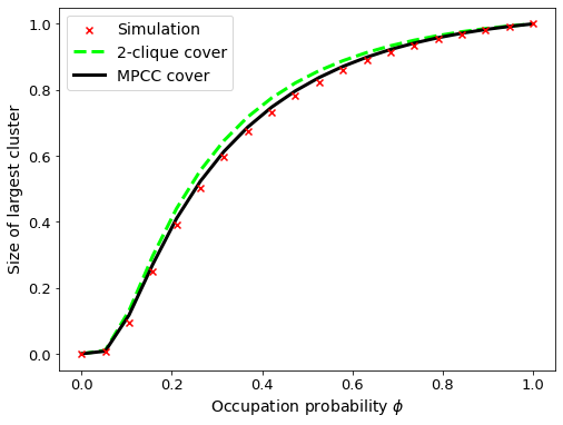
Following this, we will extract all cliques from the network and re-run the message passing equations. Finally, once our data is collected, we will visualise the theoretical results.
# Extract the MPCC clique cover (all size cliques allowed) using gcmpy
G = gcmpy.MPCC(G)

# create an instance of the MessagePassing class.
MP = MessagePassing('NULL', G, {})
MP._MPM = MessagePassingMixin('NULL', G)

# perform the experiment! (go make a cup of tea for this one ... )
GCC_all_cliques = Parallel(n_jobs=-1)(delayed(MP.theoretical)(phi) for phi in tqdm(np.linspace(0,1,20)))
# plot the results
ax = plt.figure(figsize=(8,6),linewidth=7).gca()
ax.scatter(np.linspace(0,1,len(largest_component_size)),
           largest_component_size,marker='x',color='r',zorder=100,label='Simulation')


ax.plot(np.linspace(0,1,len(GCC_2_cliques)), GCC_2_cliques,'--',linewidth=3,color='lime',label='2-clique cover')
ax.plot(np.linspace(0,1,len(GCC_all_cliques)), GCC_all_cliques, linewidth=3,color='k',label='MPCC cover')

plt.xlabel(r'Occupation probability $\phi$',fontsize=14)
ax.set_ylabel('Size of largest cluster',fontsize=14)
ax.tick_params(axis='both', which='major', labelsize=13)
plt.legend(fontsize=14)

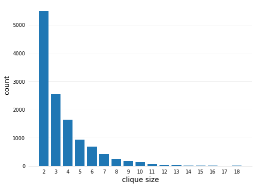
The 2-clique cover does not capture the experimental results very well. Allowing larger cliques into the cover yields a better model of the empirical network, but it still isn’t 100% capturing the connectivity of the empirical network. We will investigate the role that clique covers play in future posts!
# iterate the edges and record the clique size
cliques = {}
for e in G.edges():
    label = G.edges[e[0],e[1]]['clique']
    size = int(label.split('-')[0])
    cliques[size] = cliques.get(size, 0) + 1

for size in cliques:
    cliques[size] /= size
ax = plt.figure(figsize=(8,6),linewidth=7).gca()

ax.bar(cliques.keys(), cliques.values())
ax.set_xticks(range(2, max(cliques.keys())+1))

# visualisation stuff ...
ax.spines['top'].set_visible(False)
ax.spines['right'].set_visible(False)
ax.spines['left'].set_visible(False)
ax.spines['bottom'].set_color('#DDDDDD')
ax.tick_params(bottom=False, left=False)
ax.set_axisbelow(True)
ax.yaxis.grid(True, color='#EEEEEE')
ax.xaxis.grid(False)

plt.xlabel('clique size',fontsize=14)
plt.ylabel('count',fontsize=14)

References
[1] M. E. J. Newman, “The structure of scientific collaboration networks,” Proceedings of the National Academy of Sciences, vol. 98, no. 2, pp. 404–409, 200
[2] P. Mann & S. Dobson. Belief propagation on networks with cliques and chordless cycles (in preparation, 2022)
[3] P. Mann, V. A. Smith, J. B. O. Mitchell, and S. Dobson, “Degree correlations in graphs with clique clustering,” Phys. Rev. E, vol. 105, p. 044314, Apr 2022
[4] G. Burgio, A. Arenas, S. Gomez, and J. T. Matamalas, “Network clique cover approximation to analyze complex contagions through group interactions,” Communications Physics, vol. 4, no. 1, 2021
[5] F. Harary and E. M. Palmer, Graphical enumeration. Academic Press, 1973.
[6] https://github.com/giubuig/DisjointCliqueCover.jl